


Originally published in French in June 2018. Read the French version. Screenshots and charts are in French.
This article covers the first part of my talk at SEO Camp Day Lyon 2018. Formulas are given here with their English Excel names; the screenshots come from a French version of Excel.
Excel is an essential tool for anyone working on a computer, and especially for SEOs, who handle a lot of data. Excel can save real time, provided you know the key formulas and, above all, how to use them. The first part of the talk covered the Excel basics: simple, but worth mastering before moving on to more advanced tools.

Contents:
CONCATENATE: rebuilding full URLs after an export
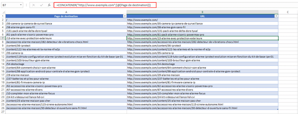
In SEO, depending on the tool used to export data, URLs can come in different formats (with or without the domain, in particular), especially in exports from Google Analytics and log files. The CONCATENATE formula reshapes URLs to make them consistent. You can then bring together data from different sources (Google Analytics, Google Search Console, Majestic, Semrush) with a VLOOKUP formula.
In practice, how do you do it?
=CONCATENATE("http://www.example.com",[@[Landing page]])http://www.example.com: first value of the string.
[@[Landing page]]: cell holding the end of the URL.
VLOOKUP: bringing data together from different sources
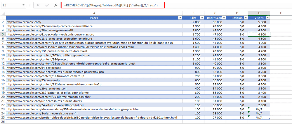
Once all the URLs exported from the different sources share the same format, they can be gathered in a single table. This is where VLOOKUP comes in: it fetches data from table B into table A. In one table you can then bring together visits, backlinks, number of rankings and so on. That lets you correlate several tables by putting related data on the same row.
In practice, how do you do it?
=VLOOKUP([@Pages],TableGA[[URL]:[Visits]],2,FALSE)[@Pages]: the value looked up (here, the full URL).
TableGA[[URL]:[Visits]]: where to search (here, the table of visits exported from Google Analytics).
2: number of the column holding the data to fetch (here, visits are in the second column of the selection).
FALSE: do not allow an approximate match.
Pivot table: grouping the data in a table
A pivot table sorts a lot of data without rebuilding tables by hand each time. The data is summarised so it can be analysed, then turned into a chart that is easier to read. A pivot table also applies filters automatically. It brings together all the information sharing a common denominator, to help you find answers.
Here is a semantic analysis where I gathered keywords about security cameras, sorted by category and sub-category. The pivot table groups the keywords by category and sub-category, and a linked pivot chart makes it concrete.
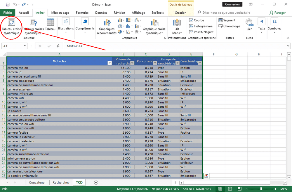
To start, in Excel, click PivotTable in the Insert tab and choose where to place it. By default, the table is inserted in a new sheet.
Fields are arranged by drag and drop. Adding several rows builds a nested table with a hierarchy between values; the order of the rows sets that hierarchy. Fields added to Values are the ones displayed in the columns.
Here I put the feature group first and the feature second, so that features are nested inside their groups. Then I put search volume and competition in Values, to weigh search volume against the average competition of each semantic field.
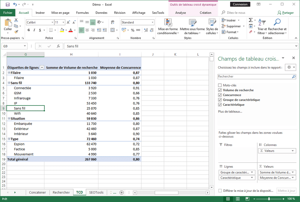
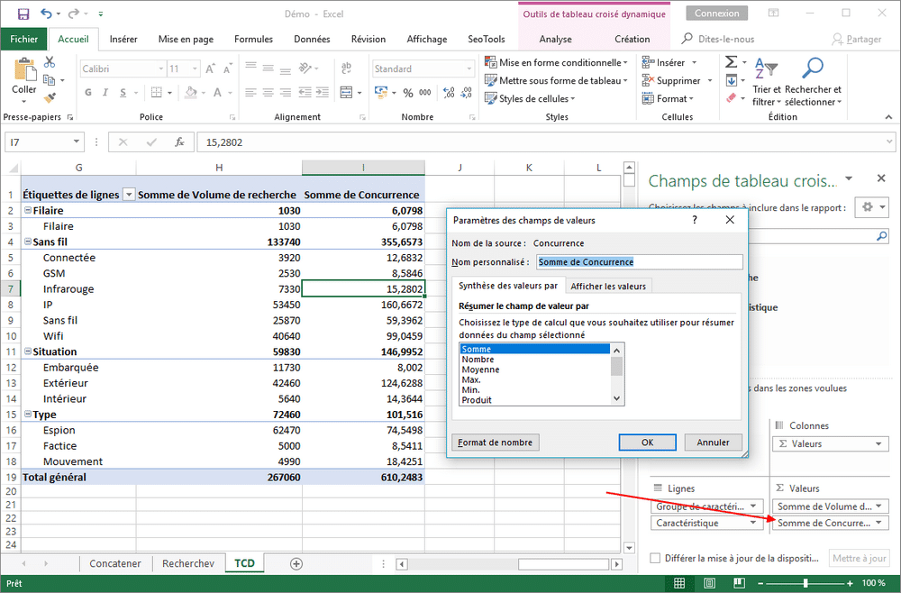
You can change the default value type chosen by Excel by clicking Value Field Settings. Here, for example, I replaced the sum of competition with its average, which makes more sense for this data.
You can also get back to the source data at any time by double-clicking a row. For example, to list every keyword in the dashcam topic, just double-click it. The keywords appear in the pivot table and can be hidden again by clicking the minus sign next to the topic.
Pivot chart: illustrating the pivot table for the client
Once the pivot table is done, you can link it to a pivot chart to make the data more visual, especially if it is meant for a client.
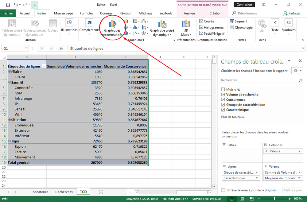
Select the pivot table and click Recommended Charts in the Insert tab. Then pick the right chart for the data: for this semantic analysis, I chose a combo chart with a secondary axis for my second metric, competition.
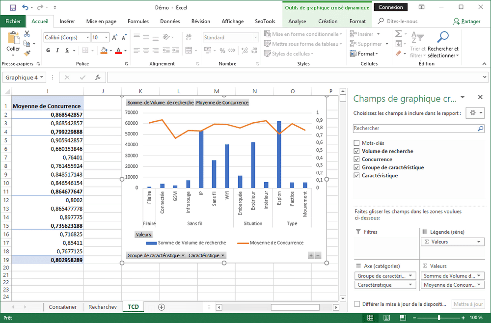
The chart is ready, and if the source table changes, the pivot table and pivot chart follow once the data is refreshed.
You get a visual result that lets you draw conclusions straight away. In this semantic analysis, the most interesting topics to work on for SEO are IP cameras and spy cameras. Competition on the second axis puts search volume into perspective.
That covers the Excel basics. For log analysis done with these same tools, read the 6 decisive SEO criteria.